
- The seasonal effect that equities do better from November through April is well-known. Here we provide a rigorous statistical test of this and a trading strategy to profits from it.
- From 1960 the S&P 500 with dividends returned on average 1.92% for the six months May to October, the “bad-periods”, while the “good-periods”, November to April, returned 8.47% on average.
- Statistics provide a 65% probability that good-periods will produce higher returns than the average of all good- and bad-periods, and a similar probability that the bad-periods will produce lower returns.
- This anomaly can be exploited by tactically shifting from more aggressive “good-period portfolios” to lower risk portfolios at the end of every April, and reversing the process end of October.
- Switching accordingly between the S&P 500 and 10-Year Treasuries would have provided an annualized return of 12.1% from 1960 to 2019 versus 9.4% for buy-and-hold the S&P 500.
A long term study supporting the seasonal observation can be found here. A related switching strategy model with cyclical and defensive ETFs is described here.
The seasonality of the S&P 500 is easily verified by backtesting with historic data. The S&P 500 with dividends from 1960 onward returned on average 1.92% for the yearly six-month periods May through October, the “bad-period”. For the other six months, the yearly “good-period”, from November through April, the average return was 8.47%.
This seasonal effect can be exploited for higher returns by investing more aggressively during the good-periods, and more defensively during the bad-periods.
Quantifying stock market seasonality
More rigorous than observing is to statistically demonstrate that the six months from November to April are usually good-periods for equities. The null hypothesis H0 is the default position, namely that there is no difference between the average returns of the good-periods and bad-periods, the average return hereinafter referred to as the “H0-return”.
In evidence-based medicine, likelihood ratios are used to assess the reliability of a diagnostic test. In finance, likelihood ratios can quantify the reliability of a financial test as well. For example, one can check the dependability of a recession indicator, as described here, or determine the probability of equities performing better over a particular period in the year depending on the outcome of a relevant diagnostic test.
Diagnostic test:
- Positive outcome = the period return is greater than the H0-return.
- Negative outcome = the period return is less than the H0-return.
The test period, from January 1960 to April 2019, held 59 cyclical good-periods and 59 cyclical bad-periods for stocks, totaling 118 six-month periods, and showed an average return of 5.20% for all periods, the H0-return.
The diagnostic test can provide the following four outcomes, depending on the actual return for a period and its magnitude relative to the H0-return, namely the number of periods in the good-period group that test positive (a) and negative (b); and the number of periods in the bad-period group that test positive (c) and negative (d).
How often those four conditions occur over the observation period are the raw data for the analysis, shown in the Table-1 for this specific investigation.
| Table 1 (Data 1960-2019) | |||
| Good Period | Bad Period | ||
| Test Result |
Positive | True Positive (a) 39 |
False Positive (c) 21 |
| Negative | False Negative (b) 20 |
True Negative (d) 38 |
|
The statistics from the test provide a 65.0% probability that the good 6-month periods from November to April produce higher returns than the H0-return of 5.20%, and a 65.5% probability that the bad 6-month periods from May to October will produce lower returns than the H0-return.
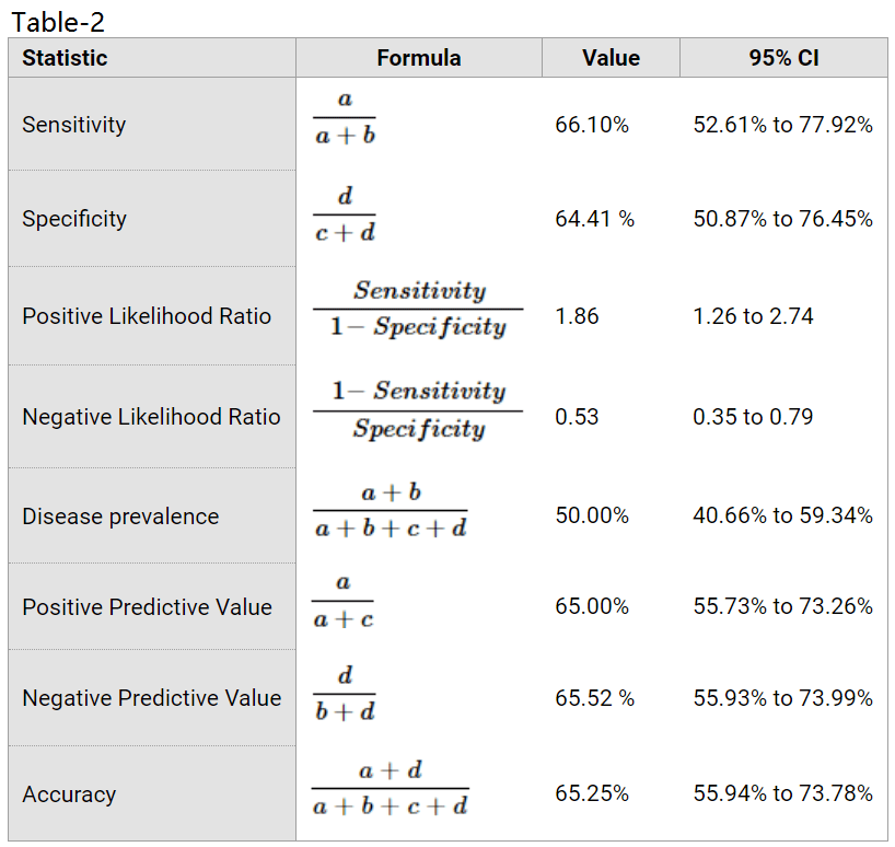
This on-line diagnostic test calculator, using the input data of Table-1 gives statistics with 95% confidence intervals, as listed in Table-2. Definitions of the various statistical terms are on the linked website.
The positive likelihood ratio is 1.86 with a 95% confidence interval of 1.26 to 2.74; a value greater than 1 produces a post-test probability which is higher than the pre-test probability (the “disease prevalence” in the statistics below, in our case the “good-period prevalence”).
The positive predictive value in the statistics (another name for the positive post-test probability) is 65% with a 95% confidence interval of 55.7% to 73.3%, denoting statistical significance because the lower confidence level of 55.7% is higher than the pre-test probability of 50.0%.
Profiting from stock market seasonality
A strategy to profit from seasonality based on the statistical odds is to have more aggressive investments during the good-periods, and more defensive ones during the bad-periods.
Because there is a 65% chance to beat the average return over the good-periods, the strategy always invest in the S&P 500 from November to April. From May to October three alternatives were investigated: 100% fixed-income, 50% equity and 50% fixed-income, and cash only without interest.
Below list the five alternatives considered. Models A, B, and E follow a seasonally variable allocation strategy, while C and D are fixed allocation models. Annualized returns are shown in brackets.
- 100% bonds (10-Year Treasuries) during the bad period (12.1%)
- 50% bonds and 50% stocks during the bad period (11.1%)
- 100% stocks (buy-and-hold) all periods (9.4%)
- 60% stocks and 40% bonds all periods (8.6%)
- 100% cash without interest during the bad period (8.0%)
Prices since 1960 for the S&P 500 with dividends and 10-Year Treasuries were derived from various sources; see the Appendix.
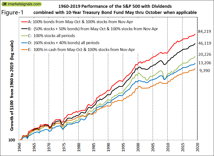
The performance over 59 years from May-1960 to April-2019 for the five alternative models is shown in Figure-1, with data plotted at six-month intervals. All trading was assumed to occur at the end of the last week of April and October.
Model A shows the highest performance, $100 would have grown to $84,219 equivalent to an annualized return of 12.1%, while Model C (buy-and-hold equity) would have produced only $20,226 for an annualized return of 9.4%.
The typical retirement savings strategy of holding 60% stocks and 40% bonds (Model D) is also one of the poor performers; $100 would have grown to $13,206 equivalent to an annualized return of only 8.6%.
For the more recent performance of the seasonal SPY-IEF switching strategy, from Jan-2000 to Apr-2019, see Figure-2 in the Appendix.
Annualized returns over consecutive 20-year periods for Models A, B, and C are listed in Table-3. It is evident that it would always have been more profitable, even during the period 1960-1983 of rising interest rates, to have some fixed-income investment during the bad-periods from May thru October. Over any of the nine periods Model A always produced the highest return.
| Table- 3 | ||||
| Period | Annualized Returns | |||
| From | To | Model A | Model B | Model C |
| 4/25/1960 | 4/25/1980 | 9.76% | 9.11% | 8.15% |
| 4/25/1965 | 4/25/1985 | 9.13% | 8.28% | 7.19% |
| 4/25/1970 | 4/25/1990 | 12.70% | 11.17% | 9.39% |
| 4/25/1975 | 4/25/1995 | 13.71% | 13.17% | 12.45% |
| 4/25/1980 | 4/25/2000 | 16.97% | 16.29% | 15.35% |
| 4/25/1985 | 4/25/2005 | 15.76% | 13.75% | 11.42% |
| 4/25/1990 | 4/25/2010 | 13.99% | 11.72% | 8.74% |
| 4/25/1995 | 4/25/2015 | 13.73% | 11.86% | 9.21% |
| 4/25/2000 | 4/25/2019 | 9.99% | 8.17% | 5.60% |
Conclusion
Based on the data since 1960, statistics confirm the seasonality of the stock market. The diagnostic test provides a 65% probability for the S&P 500 to perform better than average from November to April, and a similar probability to perform worse than average from May to October each year, indicating causation, namely that stock market returns increase or decrease due to seasonal effects.
Therefore, reducing equity allocation during the bad-periods and replacing it with fixed-income should be a winning strategy over the longer term.
Appendix
Historic equity and fixed-income prices
Prices for a hypothetical S&P 500 index fund come from:
- SPDR S&P 500 ETF (SPY) from 1993 to 2019,
- Vanguard 500 Index Fund (VFINX) from 1980 to 1993,
- From 1960 to 1980 daily data of the S&P 500 from Yahoo Finance with dividends taken from the Shiller CAPE data.
Price changes over the good- and bad six-month periods for a hypothetical 10-year Treasury bond fund come from:
- iShares 7-10 Year Treasury Bond ETF (IEF) from 1995 to 2019,
- Calculated from the 10-Year Treasury Rate from 1962 to 1995,
- From 1960 to 1962 calculated from the 10-Year Treasury yield of the Shiller CAPE data.
Profiting from stock market seasonality Jan-2000 to Apr-2019
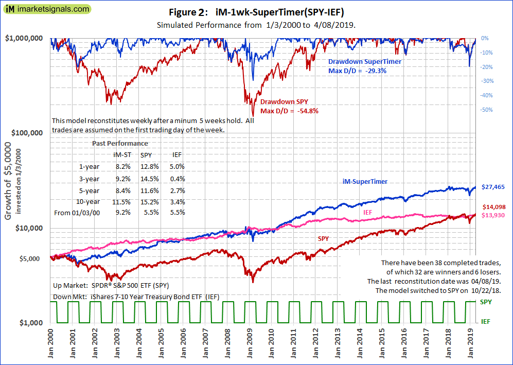
The performance of a seasonal switching strategy SPY-IEF since Jan-2000 is shown with the iM-1wk-SuperTimer in Figure-2.
The iMarketSignals’ weekly updated iM-SuperTimer defines up-market and down-market periods for stocks. It uses a combination of 15 unrelated market indicator models (including the seasonal model), all updated weekly.
For the seasonal switching strategy 14 of its component market timer models were turned off, only leaving the seasonal timer model on. Growth is plotted to a logarithmic scale, and the investment periods for stock fund SPY and bond fund IEF are depicted by the lower green graph in the figure.
Over the backtest period of more than 19 years a $5,000 initial investment would have grown to $27,465 by seasonally investing in SPY or IEF, for an annualized return of 9.2%. A $5,000 buy-and-hold investment in SPY or IEF would only have grown to about $14,000, for an annualized return of 5.5%. The maximum drawdown of -29% would also have been much better for the seasonal switching strategy model than the -55% drawdown for SPY.
(For those who are interested, the iM-1wk-SuperTimer with all the 15 component market timer models from its arsenal turned on would have produced $169,692, for an annualized return of 20.1% with a maximum drawdown of -10%. There would have been 45 completed trades, 39 of them winners.)
Hi,
I’ve reviewed your data and like the tools you’ve developed. I have some questions regarding the Seasonal Strategy (following the iM-1wk-SuperTimer).
1. Is there any reason to wait until the SuperTimer reading indicates to move into IEF to get started putting the funds to work versus putting the funds into SPY now, since its past May
2. Is there a “start up” strategy that works well with moving funds into either SPY or IEF. For example, 25% every weeks for 4 weeks(assuming the signal hasn’t changed), 25% every 2 weeks…
3. Since I’m new to your tools, can you tell me what the iM-1wk-SuperTimer will look like when it changes signals? What is in the cells to the right of the “Buys” and “Sells” cells? Is there someplace I can see examples of past readings?
Thanks, and fantastic work pulling all of this together and modeling it out.
1. The Seasonal Switching Strategy is only one of the 15 component market timers in the SuperTimer, and only has an Importance Factor of 0.5, meaning it is not very important. So there is no reason to wait to follow the signals from the SuperTimer.
2. The start-up strategy is up to users. We have no recommendations in this regard.
3. The SuperTimer signals investment in stocks when the iM-Stock Market Confidence Level iM-SMC > 50%. Historic weekly levels and holding periods can be download here:
im-smc_to_3-18-2019.xlsx
Hello,
Can I please get Seasonal Switching Strategy holding during time period Oct 2018 to Apr 2019?
Thank you,
John
10/22/18 to 4/22/19 model held Consumer Discretionary Select Sector SPDR Fund (XLY)
What was the strategy holding during time period of Nov19-Apr20?
Thasks,
Hans
10/28/19 to 4/27/20 model held Consumer Discretionary Select Sector SPDR Fund (XLY)
Cheers, G