
- Forward 10-year annualized real returns of the S&P 500 Index can be determined by regression analysis using the ratio of the Shiller CAPE-ratio and its 35-year moving average (CMA-ratio).
- Currently this ratio stands at 1.21 and forecasts a 10-year annualized real return of 6.2%, which would indicate that the market as represented by the S&P 500 is not overvalued.
- Since 1979, when the CMA-ratio was within +/-5% of the current value the 10-year annualized real returns for the S&P500 that followed ranged from 4.7% to 14.6%, averaging 9.8%.
- Investing in equities for the long-haul when the CMA-ratio is at 1.50 or higher produces poor returns, as this level of the ratio signifies overvaluation of the market.
This is a follow-up article to Estimating Forward 10-Year Stock Market Returns using the Shiller CAPE Ratio and its 35-Year Moving Average, which is referred to as the “referenced article” further down.
The standard use of the Shiller CAPE-Ratio to predict stock market returns
Robert Shiller’s cyclically adjusted price–earnings ratio, or CAPE-ratio, has served as one of the best forecasting models for long-term future stock returns.
The CAPE-ratio is calculated by dividing the average monthly price of the S&P 500 Index by the average of the last 120 months of as reported 12 month earnings per share of the S&P 500 Index, with earnings and stock prices measured in real terms. The regression equation resulting from regressing 10-year real stock returns against the CAPE-ratio has a high enough coefficient of determination (R-squared) to indicate that the CAPE-ratio is a significant variable to predict long-term equity returns.
CMA-Ratio; the CAPE-MA35 Ratio
As discussed in the referenced article, a superior method to the standard use of the Shiller CAPE-ratio is to predict 10-year real returns using the CMA-ratio as a valuation measure, which is simply the value of the Shiller CAPE-ratio divided by the corresponding value of its 35-year moving average.
Estimating forward stock market returns with the CMA- Ratio
Nobody knows the short term direction of the market in advance, but for the longer term the Shiller CAPE-ratio’s derivative, the CMA-ratio, is an excellent tool to estimate forward returns for equities.
The monthly data of Shiller’s S&P series starts in 1871, and the first value of the CAPE-ratio is available 10 years later. Therefore, the first value of the 35-year moving average of the CAPE-ratio, and thus the value of the CMA-ratio, is only obtainable 45 years after the series’ start date, in Jan-1916.
This model’s forecast estimates are based on annual regression analyses on the available point-in-time data of observed 10-year annualized real returns for the S&P 500 with dividends and corresponding CMA-ratios. Unlike in the referenced article, this analysis does not distinguish between falling and rising CMA-ratios for the yearly regression analyses.
The most recent Jan-2019 regression equation to estimate forward returns for 2029 is based on the monthly dataset from Jan-1916 to end of Dec-2008 and will be used until the end of 2019, because a new equation will apply for 2020 which will be calculated from a dataset extended by one year
It is reasonable to assume that as more historic data becomes available for the regression analyses the return forecasts should also become more robust. Equally, when less historical data was available then the forecasts would have been more tentative. Therefore Figure-1 does not include forward return estimates for earlier dates than what is shown. Note that the Jan-1979 estimate is based on the 1916-1968 dataset, and the last estimate from Jan-2019 uses the regression equation applicable to the much larger 1916-2008 dataset.
In Figure-1 the blue graph shows the actual forward 10-year annualized real returns from the S&P 500 Index with dividends. The last actual 10-year return available is 12.1% for the period Jan-2009 to Jan-2019, and this value is therefore plotted for the Jan-2009 date.
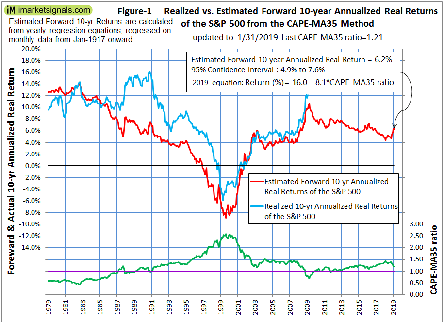
The red graph depicts the estimated forward 10-year annualized real returns obtained from regression analyses, which in Jan-2009 was 9.8%; this value is therefore also plotted for the Jan-2009 date. So an investor would have known in Jan-2009, when the CMA-ratio stood at 0.79 (the green graph at the bottom of Figure-1), that the odds were in favor of getting good returns from equities over the next 10 years.
Currently, for the 10-year period Jan-2019 to Jan-2029, the most recent regression analysis predicts an annualized real return of 6.2% despite the high likelihood of a recession during this period. (See the Appendix for the regression equation.) Whether this prediction holds up will only be known in 10 years. Note, that onward from 1983 predicted returns were mostly lower than the actual returns.
Let’s look at the CMA-ratio for 1999 which had a high value of about 2.50 then. Based on this value the 10-year forecast applicable to Jan-2009 was -6.3%. The actual 10-year annualized return from Jan-1999 to Jan-2009 was -3.8%. So, the regression analysis done in Jan-1999 with a dataset ending 10 years earlier produced a good forecast. Armed with this tool, an investor would have known in 1999 that stocks were overvalued at the time and chances were low to obtain a good return over the following 10 years.
Then, in Jan-2003 the stock market appeared reasonably priced again when the CMA-ratio had a value of 1.27 (similar to the current Jan-2019 value of 1.21). Based on this value the 10-year forecast applicable to Jan-2013 was +5.1%. The actual 10-year annualized return from Jan-2003 to Jan-2013 was +4.3%, despite the large drawdown during the 2008-09 “Great Recession”.
Historic forward stock market returns from the CMA- Ratio
Table-1 below shows average estimated forward 10-year annualized real returns for CMA-ratios ranging from 0.50 to 2.70 and also the corresponding average actual 10-year returns recorded from Jan-1949 to Dec-2008.
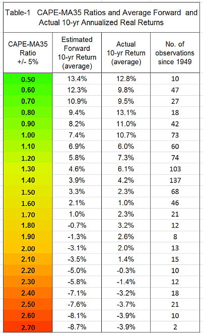
It is apparent from the table that investing in stock market funds for the long-haul when the CMA-ratio is at 1.50 will produce poor returns, as at this level and higher the ratio signals that the stock market is overvalued.
Good returns should be achievable when the CMA-ratio level stands at 1.0 or lower, as these levels of the ratio indicate that stocks are undervalued.
Realized 10-year annualized real returns for ETF (IEF) and the S&P 500
In Figure-2 the realized 10-year annualized real returns for the iShares 7-10 Year Treasury Bond ETF (IEF) (red graph) are compared to the returns from the S&P 500 with dividends (blue graph). (The ETF’s prices are adjusted for dividends and come from Portfolio123 which reconstructed daily prices for IEF prior to its inception date back to Dec-1994 from its proxy, the BofA Merrill Lynch 7-10 years US Treasury Index.)
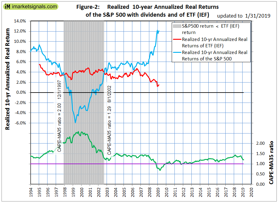
An investment made 10 years ago in ETF (IEF) returned only 1.5% after inflation to Jan-2019, while the same investment in the S&P 500 returned about 12.0%, also after inflation. Clearly the Treasury ETF was not a good investment if bought in Jan-2009 and held for 10 years.
The shaded area of the figure indicates when the 10-year forward returns for the S&P 500 were lower than for ETF (IEF), and also mark the corresponding CMA-ratios. During this period it would have been better to invest in the Treasury ETF than in equities.
A reasonably good long-term investment strategy stemming from the foregoing investigation would be to invest in
- 100% stocks when CMA-ratio < 1.20,
- 50% stocks & 50% bonds when CMA-ratio > 1.20 & < 2.00,
- 100% bonds when CMA-ratio > 2.00.
Conclusion
When many avoided the stock market during and after the 2008-09 financial crises, the then prevailing low CMA-ratios with values less than 1.0 were signaling good buying opportunities for stocks. Since 1979, there were 116 months representing excellent investment periods when the CMA-ratio was 1.0 and lower. The actual 10-year real annualized returns of the S&P 500 with dividends that followed ranged from 8.3% to 15.8%, and averaged 11.6%.
Currently it would appear that stocks are fairly valued. The current Jan-2019 CMA-ratio stands at 1.21 and forecasts a 10-year annualized real return of 6.2%. Since 1979, there were 35 months when the CMA-ratio was within +/-5% of the current value. The actual 10-year annualized real returns that followed then for the S&P 500 with dividends ranged from 4.7% to 14.6%, and averaged 9.8%.
The latest CMA-ratio can be easily calculated from Shiller’s S&P series. It is also posted monthly on iMarketSignals with the corresponding predicted 10-year annualized real return for the S&P 500 Index with dividends.
Note, that large drawdowns are always possible during a 10-year look-ahead period. Investments can be protected by following signals from various market-timing models on our website. It is also important to know when a recession is looming, because stocks usually do poorly during recession periods. Our Business Cycle Index should provide early warning of an oncoming recession.
Disclaimer
The performance data shown represent past performance, which is not a guarantee of future results. Investment returns and portfolio value will fluctuate, and current signals from the CMA-ratio may not be as good as they were in the past.
Appendix
Figure-3 shows the most recent regression plot to estimate forward returns for 2029. It is based on the monthly dataset from Jan-1916 to end of Dec-2008.
The Jan-2019 equation is:
Estimated 10-yr Annualized Real Return = 16.0 − 8.1 × CMA-ratio (%)
The coefficient of determination R-squared is 41%, indicating that the CMA-ratio explains more than 40% of the variation of 10-year real equity returns.
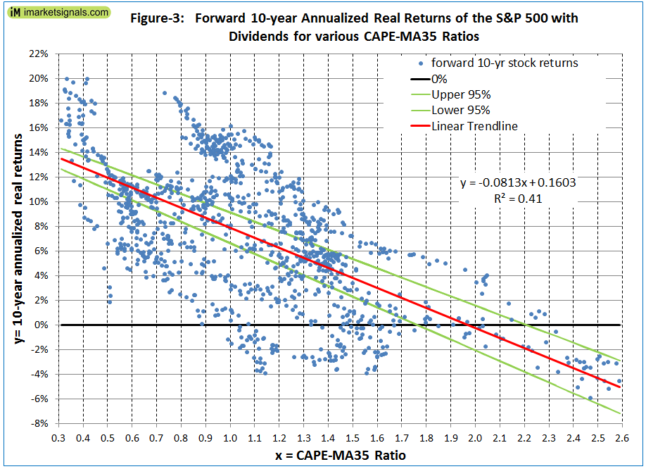
The spread of data points in Figure 3 looks pretty broad. I don’t understand why the upper and lower 95% lines are so close together unless a lot of data points are not shown.
All the monthly data points are shown. The 95% confidence lines come from the regression analysis done in excel.
-HI,
Figure 1 shows a very good predictive behaviour (except 1988-91) but it is really surprising that it can be obtained from Fig 3, where the scattering in the central region is really huge!.
I also do not understand the 95% interval, when visually it is clear that only around 25% of the points are included. ?????
The good predictive points are extreme readings (as it is usual with CAPE) but central region is really a mess. At ratio 1.1 we have a broad distribution from -4% to +16% ! The only reason I find is the long period (10 Years) that averages monthly readings.
That would be the underlying reason of using a long period, instead of 8 or 5 years, right?
Anyway it is an interesting work!
It would be very interesting to know what happens with estimations of drawdowns for the next 10 years…
You should also take into account interest rates. Higher valuations are justified under low interest rate regimes and vice versa.
We are estimating forward 10-yr annualized returns for stocks. We have no estimate of forward interest rates.