
- This is a dynamic ETF allocation strategy using the CAPE-MA35 ratio—the Shiller CAPE divided by its 35-year moving average—to identify market phases and adjust portfolio exposure.
- The model defines four primary phases with respective ETFs—Growth (QQQ), Defensive (GLD, XLU), Uptrend (QQQ, XLE), and Downtrend (GLD)—based on the trend and relative valuation of CAPE-MA35. ETF allocations are adjusted monthly in response to these phases.
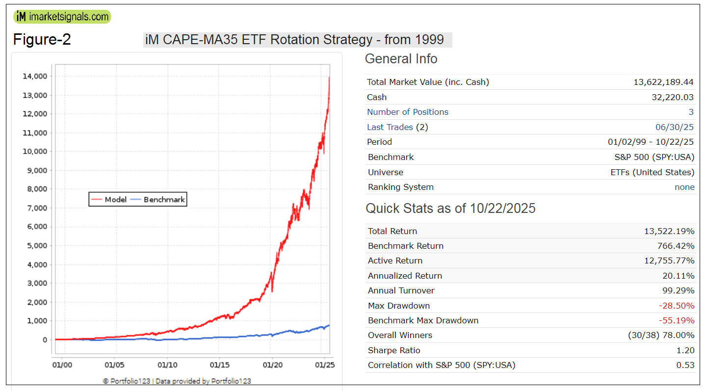
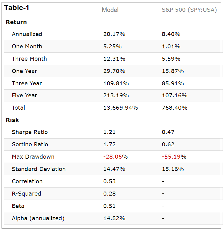
- Backtesting from 1999 to 2025 shows the model outperforms SPY with 20.1% annualized returns, lower drawdowns, and consistent long-term performance with low turnover.
- The strategy offers a practical, rules-based approach to market timing, blending long-term valuation with trend analysis for superior risk-adjusted returns.
1. Concept and Methodology
The concept and methodology were first presented here, utilizing portfolio allocations with unique ETF quantities, ranging from one to five, corresponding to each respective market phase, thereby enabling the identification of the five possible market phases by the number of positions. In this study, we present a model that maintains a portfolio of one, two, or three ETFs, achieving comparable performance
1.1 The Shiller CAPE and Its Limitations
The Shiller CAPE (Cyclically Adjusted Price-to-Earnings ratio), or P/E10, measures market valuation by dividing the inflation-adjusted price of the S&P 500 by its average inflation-adjusted earnings over the prior ten years. While CAPE is useful for estimating long-term expected returns, it performs poorly as a short- or medium-term market-timing tool due to its slow mean reversion and structural changes in markets over time.
1.2 The CAPE-MA35 Ratio
Introduced by us in 2019, the CAPE-MA35 improves upon traditional CAPE analysis by normalizing CAPE relative to its own 35-year moving average. This adjustment allows the ratio to adapt to evolving macroeconomic conditions-such as changing interest rate regimes, globalization effects, and technological shifts-thereby offering a valuation metric that better reflects current structural dynamics rather than a fixed historical mean. However, CAPE-MA35 alone is not suitable for market timing; it requires a framework that integrates both valuation level and trend behavior.
2. Market-timing Model Using CAPE-MA35
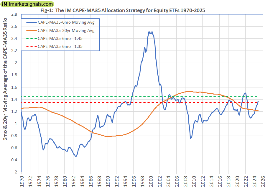
The model uses monthly S&P 500 CAPE data (point-in-time) to calculate CAPE-MA35. Two moving averages are computed: a 6-month average to identify short-term valuation trends and a 20-year (240-month) average to represent the long-term structural baseline. Two horizontal thresholds at 1.35 and 1.45 further classify valuation regimes. (Figure-1)
3. Defining Market Phases
A linear regression trend (10-month window) is applied to the 6-month moving average of CAPE-MA35. A R2 value of 0.8 is specified to validate fit of the regression line. The regression slope defines the trend direction: Slope > +0.01 indicates an Uptrend, and Slope < -0.01 indicates a Downtrend. Based on this slope and the relative position of CAPE-MA35, the market is classified into one of five phases:
| Phase | Description | ETF Allocations |
| 1. General Downtrend | Declining CAPE-MA35-6mo:Slope < -0.01 | (GLD) (1 position) |
| 2. Uptrend (Booming Growth) | Rising CAPE-MA35-6mo: Slope > +0.01, and above long-term average, and CAPE-MA35-6mo > 1.45. | (QQQ), (XLE) (2 positions) |
| 3.a Growth | Low valuation (CAPE-MA35-6mo < 1.35) and below long-term average | (QQQ) (1 position) |
| 3.b Defensive | Very high valuation (CAPE-MA35-6mo ≥ 1.45) and above long-term average | (XLU), (GLD) (2 positions) |
| 3.c Growth + Defensive | (CAPE-MA35-6mo > 1.35) and below long-term average, OR (CAPE-MA35-6mo < 1.45), and above long-term average | (QQQ), (XLU), (GLD) (3 positions) |
4. Portfolio123 Implementation Logic
The model is implemented in Portfolio123 using nested eval() functions. In plain language, the allocation logic is:
- If the CAPE-MA35 6-month SMA trend slope < -0.01 → Downtrend portfolio, otherwise
- If the CAPE-MA35 6-month SMA > its 20-year average and >1.45, and slope > +0.01 → Uptrend portfolio, otherwise
- If the CAPE-MA35 6-month SMA is below its 20-year average: and <1.35 → Growth portfolio; otherwise → (Growth + Defensive) portfolio. If it is not below its 20-year average: and <1.45 → (Growth + Defensive) portfolio; otherwise if ≥1.45 → Defensive portfolio.
5. Backtest and Results (1999-2025)
Backtesting from January 1999 through October 2025 was conducted on Portfolio123, which also provides extended ETF proxies for pre-inception data. A transaction cost of 0.1% per trade was applied.
Results Summary:
- Annualized return: 20.1%
- Maximum drawdown: -28%
- Total realized trades: 35 (27 profitable)
- Shortest holding period: 28 days
- Average annual turnover: ≈100%
Compared with SPY, the model demonstrates lower volatility and drawdown, approximately 18× higher cumulative return, and consistent long-term performance with low trading activity. (Figure-2 and Table-1)
6. Discussion
The CAPE-MA35 framework integrates long-term valuation awareness with short-term trend analysis to enhance tactical allocation decisions. Unlike static CAPE-based valuation strategies, it adjusts dynamically to market structure changes and macroeconomic evolution. Although based solely on publicly available CAPE data, its combination with systematic ETF rotation, using only 4 ETFs, achieves high risk-adjusted performance and a stable allocation regime.
7. Conclusion
The Dynamic ETF Allocation using CAPE-MA35 provides a practical market-timing approach that bridges long-term valuation context and medium-term trend signals. Its performance since 1999 demonstrates that valuation-informed, trend-adaptive strategies can outperform passive benchmarks while managing downside risk and turnover efficiently.
8. Following the Model
The model will be updated weekly for Silver subscribers. All trades since inception to 9/22/2025 are listed in the Excel file: iM-CAPE-MA35-Transactions.xls freely downloadable to all. The current holdings are GLD, QQQ and XLU equal weighted, since 6/3/2024.
APPENDIX
A. Investment Phases 1999 to 2025
| iM CAPE-MA35 Rotation Strategy Investment Phases with R2>0.8 (1999-2025) |
|||
| start date | Investment Phase | Length | |
| Cycle | end date | Type | (days) |
| 1 | 1/4/1999 | Defensive | 210 |
| 8/2/1999 | |||
| 2 | 8/2/1999 | Uptrend | 154 |
| 1/3/2000 | |||
| 3 | 1/3/2000 | Defensive | 399 |
| 2/5/2001 | |||
| 4 | 2/5/2001 | Downtrend | 609 |
| 10/7/2002 | |||
| 5 | 10/7/2002 | Defensive | 28 |
| 11/4/2002 | |||
| 6 | 11/4/2002 | Growth+Defensive | 28 |
| 12/2/2002 | |||
| 7 | 12/2/2002 | Downtrend | 217 |
| 7/7/2003 | |||
| 8 | 7/7/2003 | Growth | 147 |
| 12/1/2003 | |||
| 9 | 12/1/2003 | Growth+Defensive | 126 |
| 4/5/2004 | |||
| 10 | 4/5/2004 | Uptrend | 154 |
| 9/6/2004 | |||
| 11 | 9/6/2004 | Defensive | 28 |
| 10/4/2004 | |||
| 12 | 10/4/2004 | Growth+Defensive | 728 |
| 10/2/2006 | |||
| 13 | 10/2/2006 | Growth | 91 |
| 1/1/2007 | |||
| 14 | 1/1/2007 | Growth+Defensive | 462 |
| 4/7/2008 | |||
| 15 | 4/7/2008 | Growth | 28 |
| 5/5/2008 | |||
| 16 | 5/5/2008 | Downtrend | 518 |
| 10/5/2009 | |||
| 17 | 10/5/2009 | Growth | 882 |
| 3/5/2012 | |||
| 18 | 3/5/2012 | Downtrend | 91 |
| 6/4/2012 | |||
| 19 | 6/4/2012 | Growth | 1372 |
| 3/7/2016 | |||
| 20 | 3/7/2016 | Downtrend | 119 |
| 7/4/2016 | |||
| 21 | 7/4/2016 | Growth | 609 |
| 3/5/2018 | |||
| 22 | 3/5/2018 | Growth+Defensive | 308 |
| 1/7/2019 | |||
| 23 | 1/7/2019 | Growth | 84 |
| 4/1/2019 | |||
| 24 | 4/1/2019 | Downtrend | 189 |
| 10/7/2019 | |||
| 25 | 10/7/2019 | Growth | 364 |
| 10/5/2020 | |||
| 26 | 10/5/2020 | Downtrend | 28 |
| 11/2/2020 | |||
| 27 | 11/2/2020 | Growth | 91 |
| 2/1/2021 | |||
| 28 | 2/1/2021 | Growth+Defensive | 217 |
| 9/6/2021 | |||
| 29 | 9/6/2021 | Uptrend | 210 |
| 4/4/2022 | |||
| 30 | 4/4/2022 | Defensive | 63 |
| 6/6/2022 | |||
| 31 | 6/6/2022 | Growth+Defensive | 91 |
| 9/5/2022 | |||
| 32 | 9/5/2022 | Downtrend | 301 |
| 7/3/2023 | |||
| 33 | 7/3/2023 | Growth | 336 |
| 6/3/2024 | |||
| 34 | 6/3/2024 | Growth+Defensive | |
B. Calendar Year Returns
| Calendar Year Returns (%) for iM CAPE-MA35 4-ETF Rotation Strategy |
|||
| Year | Model | Bench | Excess |
| 1999 | 22.98 | 20.39 | 2.59 |
| 2000 | 10.02 | -9.74 | 19.76 |
| 2001 | 0.00 | -11.76 | 11.76 |
| 2002 | 33.07 | -21.58 | 54.66 |
| 2003 | 19.42 | 28.18 | -8.76 |
| 2004 | 16.49 | 10.70 | 5.79 |
| 2005 | 12.56 | 4.83 | 7.73 |
| 2006 | 17.42 | 15.85 | 1.57 |
| 2007 | 23.10 | 5.15 | 17.96 |
| 2008 | 4.29 | -36.79 | 41.09 |
| 2009 | 28.04 | 26.35 | 1.69 |
| 2010 | 19.79 | 15.06 | 4.74 |
| 2011 | 3.34 | 1.89 | 1.44 |
| 2012 | 17.41 | 15.99 | 1.42 |
| 2013 | 36.03 | 32.31 | 3.72 |
| 2014 | 18.69 | 13.46 | 5.23 |
| 2015 | 9.30 | 1.23 | 8.07 |
| 2016 | 10.81 | 12.00 | -1.19 |
| 2017 | 32.18 | 21.71 | 10.47 |
| 2018 | 7.15 | -4.57 | 11.72 |
| 2019 | 51.19 | 31.22 | 19.97 |
| 2020 | 52.07 | 18.33 | 33.74 |
| 2021 | 24.37 | 28.73 | -4.36 |
| 2022 | 15.06 | -18.18 | 33.23 |
| 2023 | 16.57 | 26.18 | -9.60 |
| 2024 | 22.58 | 24.89 | -2.31 |
| 2025** | 33.59 | 16.57 | 17.02 |
| ** to 10/24/2025 | |||
Are calendar year returns since 1999 available? Thanks.
Yes, we will update the description on the site.
The calendar year returns are now listed in the Appendix. We have also listed the various investment phases.
Excellent. Thank you.
is there a way to reduce the Drawdawns, maybe adding Dollar index or some cash equivalent (BIL; SHY, BOX, short term bond)?
Very nice, one trade switch a year average, sharpe 1.2, monthly drawdown about 21.2%. The simplicity makes it more doable outside the US and, I would suggest, makes it more likely to perform well into the future. Thanks guys.
Well done, thank you, no losing calendar years. Do you guys intend to update this strategy in the blog? What’s the best way to follow signals?
Ignore questions, ….
hello, i have checked 20008 and the calculation looks wrong. you aare saying that you largelly owned gold trough 2008, but during the period the etf lost value. could you clarify?
hello, i have checked 20008 and the calculation looks strange. you aare saying that you largelly owned gold trough 2008 from may till end of the year, but during the period the etf was mostly flat? how do you justify the performance in 2008?