
- A simulation of this strategy with annual withdrawal rates of up to 10% still showed long-term growth which exceeded that of buy-and-hold the S&P 500 ETF (SPY).
- The backtests use the FactSet stock database and FactSet’s Revere Business Industry Classifications System (RBICS).
- The model holds equal-weight 10 stocks of the Russell 1000 index which are ranked with a simple ranking system to identify shares of the highest “quality” companies.
- The strategy provides a high dividend yield because a minimum yield excess (depending on RBICS sector type) over the yield of SPY is a critirium for stock selection.
- From Jan-2000 to Jun-2020 this strategy without withdrawals would have produced an annualized return (CAGR) of 21.5%, much more than the 5.6% CAGR obtained from SPY over the same period.
Investment philosophy
Unlike investments that targets companies with consistent and perennial dividends, cash needs are provided by a strategy of trading large-cap stocks with good dividends and holding them on average for six months. The simulation shows that this would not only have generated a very high dividend yield of about 3.7% (average for last 10 years), but also would have provided significant growth even for high withdrawal rates.
Performance of the RBICS sectors in the Russell 1000
This model uses the FactSet stock database and FactSet’s Revere Business Industry Classifications System (RBICS) newly available at the online portfolio simulation platform Portfolio 123 (P123).
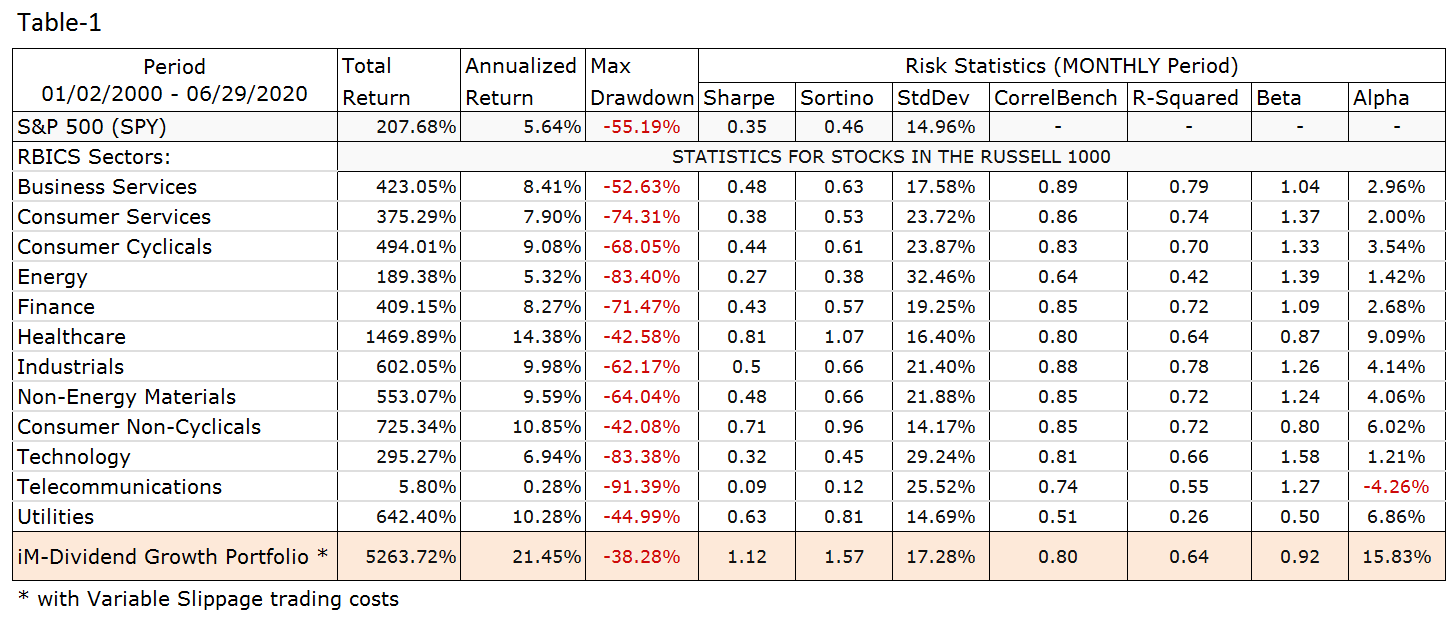
RBICS sector returns for the period Jan-2000 to Jun-2020 were determined for the P123-Russell 1000 universe in order to find the worst performing sectors so that they could be excluded from the model. Performance for each of the twelve RBICS sectors with all stocks of the sector held equal-weight is shown in Table-1 and can be compared to the performance of benchmark SPY.
Healthcare performed best, followed by Consumer Non-Cyclicals and Utilities. The worst returns came from sectors Telecommunications and Energy.
The Ranking System
The model ranks stocks from the P123-Russell 1000 universe with a modified version of the P123 ranking system “Basic-Quality”, described as follows:
Basic ranking systems are those that focus on a single well-recognized investing style. This one identifies shares of the highest “quality” companies.
The factors used in this ranking system are:
1. Profit Margins
2. Turnover
3. Returns on Capital
4. Financial Strength
Buy & Sell Rules
Subsequent to ranking the following buy rules are applied:
- Exclude stocks from the Telecommunications and Energy sectors because of poor historic sector performance, and Finance because the ranking system is not suitable for financial stocks.
- For each of the nine remaining sectors a minimum percentage yield excess over the yield of SPY is specified.
- A minimum market capitalization of $1,000-million is also required.
- Only 10 stocks are periodically selected, and there may not be more than 4 stocks from one sector among them.
- Stocks are only bought on the first trading day of the first week of a month, usually a Monday.
There are only two sell rules:
- Stocks are sold when their rank position within the ranked stocks array becomes greater than 25 (the highest ranked stock is position 1, the next is 2, etc.),
- and can only be sold on the first trading day of the first week of a month, usually a Monday.
Performance for various withdrawal rates
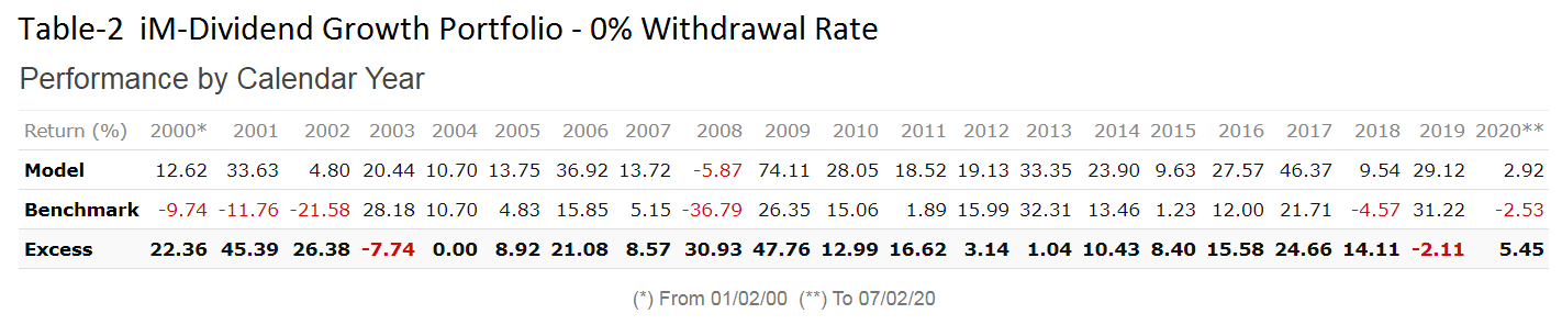
The model was originally optimized for the 15 year period starting in 2005. Subsequently the backtest period was lengthened by 5 years. Thus performance for the period 2000 to 2005 is out of sample. Backtests were performed for withdrawal rates ranging from 0% to 10%.
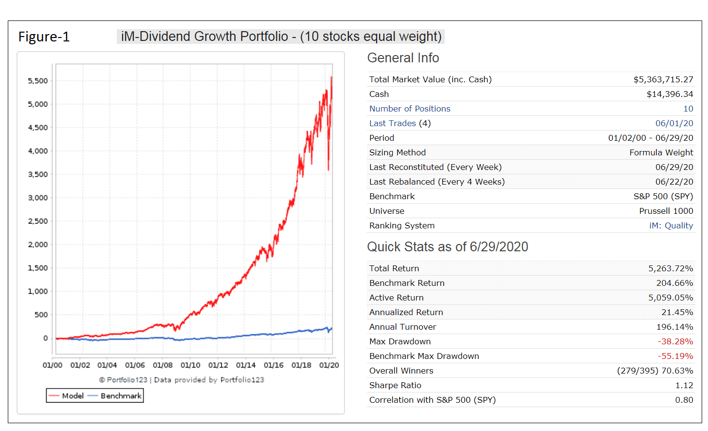
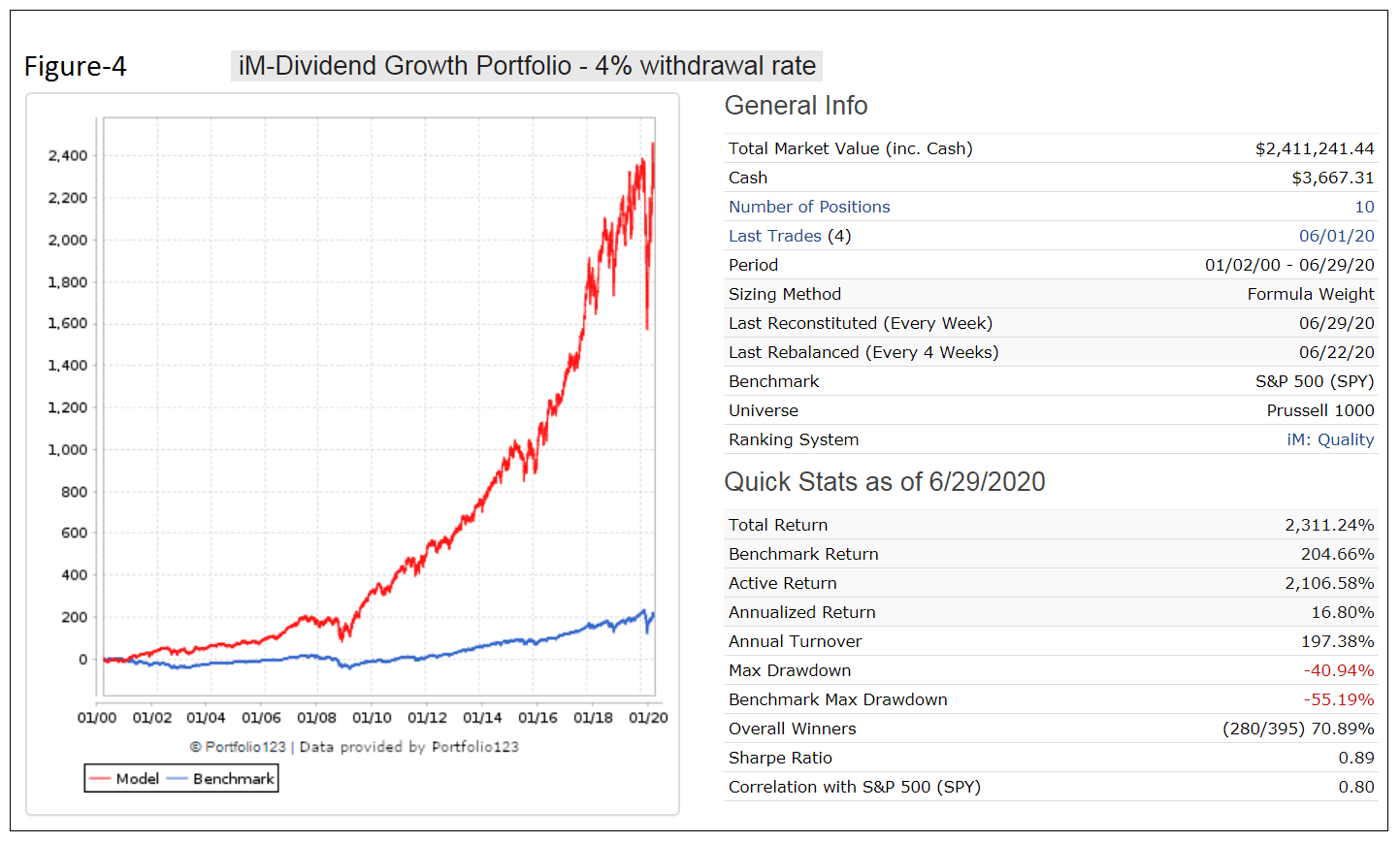
The simulated performance without withdrawals is shown in Figure-1, and the calendar year returns are in Table-2. There is no market timing involved; trading costs and slippage were assumed to be about 0.15% of each trade amount. (For performance of models with 4% and 10% withdrawal rates see Figures-4 and -5 in the appendix.)
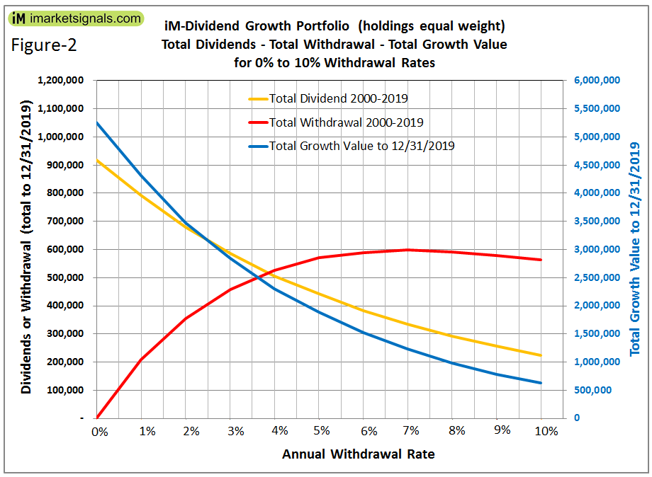
Also a withdrawal rate higher than 4% would not have increased the total withdrawal amount by much, while it would have significantly reduced the total growth amount over 20 years. For example, raising the withdrawal rate from 4% to 5% would have caused an increase of only about $43,000 in the total amount withdrawn, but would simultaneously have reduce the end portfolio value by about $420,000.
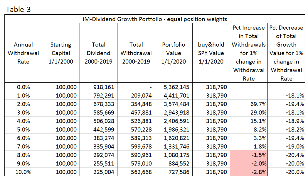
Note, that Total Growth Value is Portfolio Value minus Starting Capital.
For this model, withdrawal rates higher than 7% are counter-productive because the total withdrawal amount from Jan-2000 to Dec-2019 becomes less for rates higher than 7%. This is also graphically depicted in Figure-2 by the red graph peaking at a withdrawal rate of 7%. Also it is evident that after a withdrawal rate of 4% the red graph flattens, meaning that there is not much to be gained by withdrawing more that 4% annually. (Figure-4 and Table-4 in the appendix show performance and annual results, respectively, for a model with a 4% annual withdrawal rate.)
The blue graph in Figure-2 shows for various withdrawal rates the total growth amount over this 20-year period (right side vertical axis) to which one has to add the starting capital of $100,000 to determine the end portfolio value on Dec-31-2019.
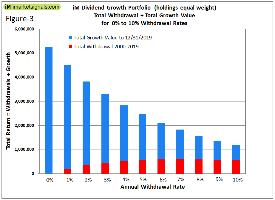
Figure-3 depicts for various withdrawal rates the total return from this portfolio, being total withdrawals plus total growth over the backtest period. The red portions of the bars represent the total withdrawals. It is evident that for 5% to 10% withdrawal rates total withdrawals do not differ by much, but growth value decreases drastically as withdrawal rate increases.
Conclusion
The analysis shows that following the iM-Dividend Growth investment strategy would have produced excellent returns, much preferable to a buy-and-hold investment strategy of stock index funds. High withdrawal rates should be possible without depleting the investment due to the high dividend yield achieved by this strategy, about 1.7-times the yield of SPY, and the exceptional growth performance.
Minimum trading is required as the rules specify this to occur only at the beginning of a month.
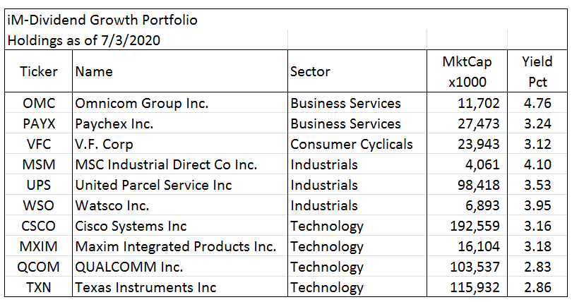
The current holdings are listed in the appendix.
At iMarketSignals one can follow this strategy where the performance will be updated weekly.
Disclaimer:
All results shown are hypothetical and the result of backtesting over the period 2005 to 2020. No claim is made about future performance.
Appendix

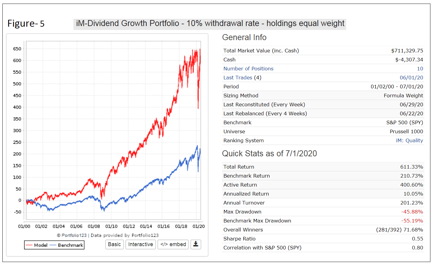
Even for a withdrawal rate of 10% this model shows a total return of about 3-times that of SPY over the backtest period.
What’s in a name?
The term “dividend growth” is normally used for companies that manage to raise their dividends on an annual base for many years in a row. The strategy doesn’t seem to concerned with dividend growth at all. Because of that it seems to be a bit of an odd name as its goal is completely different.
Of course it’s very interesting all the same! But I would probably re-phrase if published on SA or so.
drftr
The name implies that the model provides a very good dividend income and simultaneously good growth.
Never-mind what it means for a company. I have tested this model on a 100 stock universe of companies that manage to raise their dividends on an annual base for many years, but it does not nearly provide a similar high dividend yield and growth with those companies.
Also if you look at the holdings of the VDIGX Dividend Growth Fund you will find that it is not only targeting companies that have continuously raised their dividend.
Georg,
I’m confused by the data in the column MktCap X1000. In the header for the 20 year graph, it stated that there are “10 stocks, equal weight.” As an example, Watso, WSO, shows at 6,893 value, and Cisco, CSCO, shows 192,599 for the MktCap x 1000.
If I have $10,000 to invest in the 10 stocks identified, is it correct that I equal weight the purchase so the WS0 value is $1,000 and so is CSCO’s value $1,000?
This to me means you use the MktCap x 1000 to determine which stock you are picking, and I can ignore that data — all I need to do is buy $1,000 of both WS0 and CSC0. If not, indicate how I figure out how many shares of each of these two stocks I need to buy.
Market Cap is just for informational purposes and is expressed in $-millions.
WSO has a Market Cap of $6,893 x 1000 Million, or $6.893-Billion.
Equal weight means if you have $10,000 to invest, then in a 10-position model one would invest $1,000 in each position.
Hello,
congratulations for the very interesting approach and past metrics. Just un easy info, please:
in the backtest, did you take under consideration the survivorship bias on Russell 1000 stocks ?
Thanks for your attention and have a great day.
Corrado
The backtest uses the point-in-time stock holdings of the Russell 1000 as provided by Portfolio 123, meaning, for example, that when the model selected stocks in 2005 it would use the 2005 stock holdings of the Russell 1000.
Many thanks. Excellent approach.
Best regards !
Hi Georg, just 3 other questions, please.
1. Have you ever considered the idea to cover the long position with an hedged short position on S&P500 ? (let’s say: 40% short S&P and 60% long on the selected stocks).
2. Furthermore, same idea but through 1 month short naked call ATM on S&P500 or through 6/7 months OTM protective put?
3. Is it possible to get the historical serial (excel file, i.e.) of you daily mark-to-market portfolio, in order to better analyze (and, of course, to share with you) some improvement from hedging techniques ?
Thanks again and best regards,
Corrado
1. With a permanent 40% short SPY position (Margin Carry Cost=4.0%) and a 4% withdrawal rate the model still shows an annualized return of 13.1% with a max D/D=24%.
Results for a $100,000 initial investment on 1/1/2000 to 1/1/2020:
Total Dividends received = $283,538
Total Withdrawals = $361,486
Portfolio Value (1/1/2020) = $1,166,207
2. Calls and Puts cannot be modeled on Portfolio 123.
3. Daily Portfolio value is easily downloaded from P123 in excel format. But for which specific withdrawal rate would you like to have it?
Thanks, Georg.
0% withdrawal rate would be fine
best regards,
Corrado
Hi Georg and thanks for the data you kindly submitted me.
I tried 2 hedged versions:
1. A Static 40% short SPY hedged version, in which rebalancing takes place every ending year.
In this case, the average annual ROE is 10.35% (the no hedged version has 22.50%) with a max draw-down = -10.40% (versus -38.28% for the no hedged version).
Here the link with the 2 equity lines, in logarithmic scale.
https://prnt.sc/u29n36
2. A dynamic 35% short SPY hedged version, in which the hedging occur just when the VIX is above 30.
In this case, the average annual ROE is 19.85% (versus 22.50% for the no hedged version) and the max draw-down is -18.31%.
https://prnt.sc/u29i8b
For both versions, 0% withdrawal rate is supposed.
in which rebalancing takes place every year
1. For your static 40% short SPY hedged version you must have used 40% long SH which reduces the stock holdings to 60%.
If you use 40% short SPY in a margin account then stock holding remain at 100% and the annualized return would have been 17.5% and max D/D= -23%. A similar performance would be achieved by being long 40% SH bought on margin.
2. Your results for hedging with VIX>30 also assume using 35% long SH which reduces the stock holdings to 65% when the hedge is on.
CALENDAR YEAR PERFORMANCE (%)
Return … Model … SPY … Excess
2000 … 12.62 … -9.74 … 22.36
2001 … 33.63 … -11.76 … 45.39
2002 … 4.80 … -21.58 … 26.38
2003 … 20.44 … 28.18 … -7.74
2004 … 10.70 … 10.70 … 0.00
2005 … 13.75 … 4.83 … 8.92
2006 … 36.92 … 15.85 … 21.08
2007 … 13.72 … 5.15 … 8.57
2008 … -5.87 … -36.79 … 30.93
2009 … 74.11 … 26.35 … 47.76
2010 … 28.05 … 15.06 … 12.99
2011 … 18.52 … 1.89 … 16.62
2012 … 19.13 … 15.99 … 3.14
2013 … 33.35 … 32.31 … 1.04
2014 … 23.90 … 13.46 … 10.43
2015 … 9.63 … 1.23 … 8.40
2016 … 27.57 … 12.00 … 15.58
2017 … 46.37 … 21.71 … 24.66
2018 … 9.54 … -4.57 … 14.11
2019 … 29.12 … 31.22 … -2.11
YTD … 31.12 … 15.59 … 15.53
Is it still getting updates ?
When u just starting, how u adjust size of trades , at any model , thanks
The iM-Dividend Growth Portfolio is updated weekly. It is in the Bronze section of iM.
If one wants to follow the model it is best to hold all 10 positions.
Are all 10 positions brought to equal weight on a weekly or monthly basis? Or does the model conduct the buys and sells without rebalancing all of the positions?
This model buys, sells and rebalances to equal weight on the first trading day of each month.
We only report the sell and buy trades by email, but all the trades, including rebalancing trades and dividends paid, can be seen on the weekly detailed performance reports usually published on Tuesdays.