
Most of us entrust our savings to financial organizations in the belief that this will provide us with better investment results than we could have achieved ourselves. These companies advocate a buy-and-hold strategy of bond- and stock funds, charge fees, and usually perform poorly. A convenient way to improve on buy-and-hold and to do better than financial organizations is to periodically switch one’s investment from stocks to bonds and vice versa as indicated by the Moving Average Crossover MAC-system. The MAC-system (described in Beyond the Ultimate Death Cross) uses cross-overs of moving averages of the S&P 500 to determine investment periods for the stock- and bond market.
The key to this model was finding moving averages whose cross-overs have the highest probabilities of successfully signaling stock market gains or losses. I found these moving averages using likelihood ratios. The most profitable buy signals occur when the 34-day exponential moving average (EMA) of the S&P 500 becomes greater than 1.001 times the 200-day EMA. The best sell signals are generated when the 40-day simple moving average (MA) of the S&P 500 crosses below the 200-day MA.
The MAC-system has the attributes needed to make it a believable market timing model:
- it is simple, rational, and rule based,
- has very few variables (only four moving averages),
- has sufficient sample size with adequate supporting data (1950–2014),
- and it is testable.
The original study used daily data from Jan-4-1965 to Jul-6-2012. The study period has now been extended to almost 65 years, from Jan-3-1950 to May-22-2014.
Stock Market Data
Daily data for the S&P500 to determine the moving averages is from Yahoo!Finance. Dividend adjusted values of SPY, the ETF which tracks the S&P500, can be obtained from Jan-9-1993 onward. For the preceding time period to Jan-3-1950 a synthetic SPY was calculated using daily data of the S&P500 and monthly dividends from Robert Shiller’s S&P data series.
Bond Market Data
Values for IEF, the iShares 7-10 Year Treasury Bond ETF are available from July 2002 onward. From 1950 to 2002 the 10-year Treasury Note yield was used to determine bond values at start and end of bond market investment periods. Daily yield data is available from January 1962 and prior to that monthly values are from Shiller’s data series. For an example of calculating bond returns see the Appendix.
Backtest Results 1950-2014
The model generated 61 investment periods, 31 for stocks and 30 for bonds as listed in the Appendix. There were only 8 periods which produced negative returns ranging from -0.1% to -9%. For an investment made in the beginning of 1950 the return to May-22-2014 would have been 3.5 times more from the MAC-system than what buy-and-hold of SPY produced, $100 would have grown to $311,000.
| annualized return (CAGR) | |
| Buy&Hold S&P500 with dividends | 11.21% |
| MAC System (S&P500 with dividends + 10-yr bonds) | 13.39% |
| MAC-system absolute return is 3.49 times Buy&Hold |
Backtest Results 1999-2014
The model generated 13 investment periods from November 1998 to May 2014. There was only one period producing a negative return (0.26%). The absolute return of an initial investment to May-22-2014 would have been 2.4 times bigger from the MAC-system than what one would have had from buy-and-hold of SPY.
| annualized return (CAGR) | |
| Buy&Hold S&P500 with dividends | 5.33% |
| MAC System (S&P500 with dividends + 10-yr bonds) | 11.32% |
| MAC-system absolute return is 2.36 times Buy&Hold |
Backtest Results 1999-2014 using a web-based stock trading simulation site.
For this simulation the MAC-system was designed to either select IEF or TLT as the bond fund depending on which was higher ranked at the time when MAC signaled the beginning of a bond market investment period. Also the simulation results differ slightly from those of the spreadsheet calculation because the criteria were evaluated only at the end of each week and due to differences in the way exponential moving averages are calculated for the two analyses. However, returns are similar as one can see from Figure-1.
There were only 12 investment periods, all producing positive returns (Overall Winners 12/12, 100%). The simulation’s annualized return was 11.7% with a maximum draw-down of -17%. An initial investment of $20,000 made on Jan-2-1999 would have grown to $109,713 by May-22-2014, about 2.7 times what SPY buy-and-hold would have produced. Note, that the benchmark return shown in the figures below is for the S&P500, not for SPY.
Figure-1: MAC-system Jan-1999 to May-2014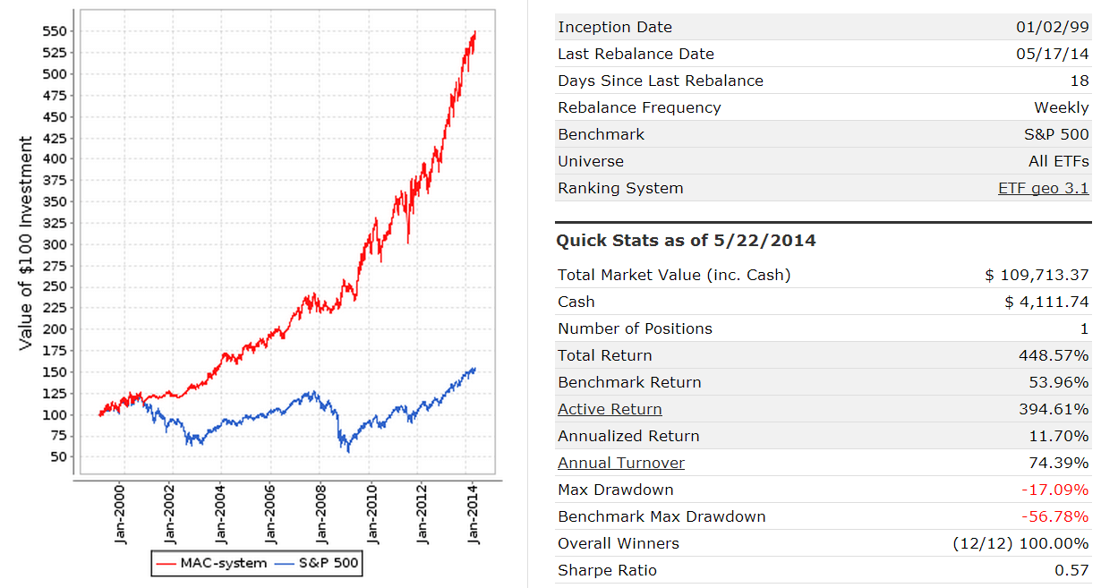 (click to enlarge)
Additional simulations with various starting and ending dates were performed. The MAC-system always avoided down-stock-market periods and followed the S&P500 during up-stock-market periods. For example, had one started the simulation at the beginning of the last recession the MAC-system would have avoided the 55% draw-down of the S&P500, as can be seen in Figure-2.
Figure-2: MAC-system Dec-2007 to May-2014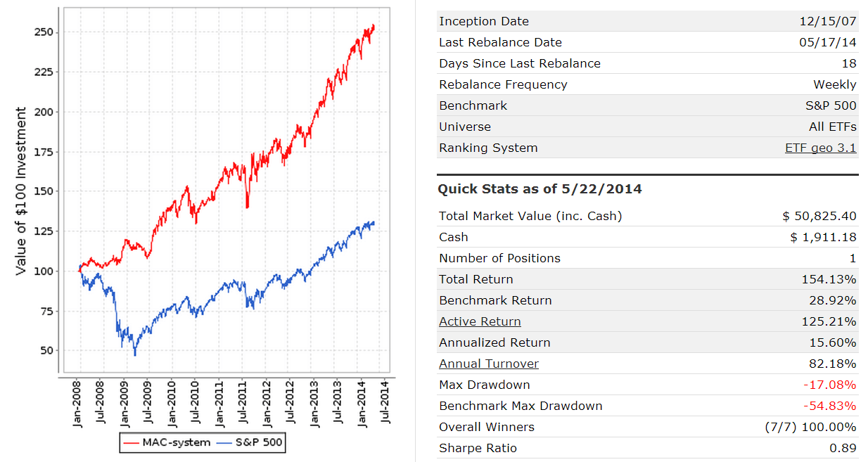 (click to enlarge)
Out-of-sample performance
The MAC-system was originally published on Jul-31-2012. Since Dec-30-2011 it has signaled a continuous investment in the stock market (SPY) and is currently still invested in SPY. The out-of-sample performance from Jul-31-2012 to May-22-2014 of SPY adjusted for dividends was 42.8% for an annualized return of 21.8%.
For the same period, a combination of two of oldest variable annuity accounts of financial service organization TIAA-CREF, 60% CREF Stock and 40% CREF Bond returned 31.9% for an annualized return of 16.6%. The lesser performance of the usually recommended 60:40 stock-bond fund combination highlights the advantage of following the MAC market timing system.
Following the MAC-system
Past performance is no guarantee of future performance. However, this model has now been backtested over almost 65 years and has performed well. How much longer must one backtest? Surely 65 years is long enough.
Weekly updates of the system are available on our website every Friday and can be viewed at no cost the following Monday evening.
Appendix
10-year Treasury Note returns
This is an approximate calculation and abbreviations are as follows:
Yo = % yield at the beginning of the investment period
Ye = % yield at the end of the investment period
C = assumed coupon = (Yo + Ye)/2 * $100
Vo = Bond Value at the beginning of the investment period (Dollars)
Ve = Bond Value at the end of the investment period (Dollars)
FV = Future Value at bond redemption = $100
In = Income from coupons (Dollars)
L = Length of investment period (years)
Po = Period to maturity at the beginning of the investment period (years)
Pe = Period to maturity at the end of the investment period (years)
PV = Present Value, the excel formula for present value is: PV(Y,P,C,FV)
Example: Bond market investment period 12/14/07 – 8/3/09
L = 1.64 years
Yo = 4,23%
Ye = 3.64%
C = (4.23 + 3.64)/2 = $3.94
Vo = PV(Yo,Po,C,FV) = PV(0.0423,10,3.94,100) = $97.67
Ve = PV(Ye,Pe,C,FV) = PV(0.0364,(10-1.64),3.94,100) = $102.13
In = 1.64 * $3.94 = $6.46
Return = ($102.13 – $97.67 + $6.46) = $10.92
Pct Return = $10.92 / $97.67 = 11.18%
Over the same period IEF adjusted for dividends returned = 11.52%
Stock- and Bond Market investment periods
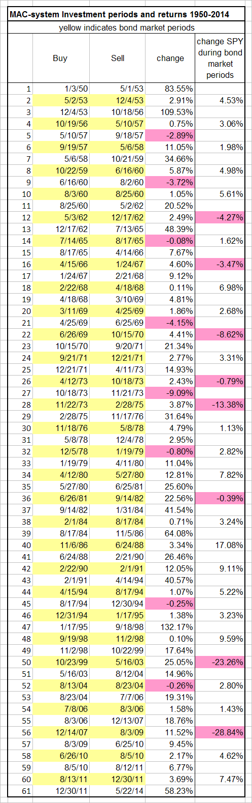
I’d love to see the S&P returns during the bond market periods of this strategy, just out of curiousity. Also, what is the max drawdown from the backtest to 1950? Do you have std dev data for any of these time periods? Thank you!
Joel, We have updated the table to show returns for S&P with dividends during MAC’s bond market periods. Adding all the returns for bonds one gets 145.86% and adding all the returns for the S&P one gets 27.31%.
Calculating maximum draw-down is a bit more difficult because we don’t have daily values of a synthetic IEF, only change in value over bond market periods, but I will give it a shot assuming that a synthetic IEF changes linearly over bond market periods, which is obviously not the case.
Thanks for posting. So the rules are when the system generates a buy go long SPY & when a sell is generated then sell SPY and invest the proceeds in TLT?
In late 2010 there was a buy signal generated yet the red/sell signal (40 period)was lower already. What if the market sold off from that point? How would we know to rotate out of SPY into TLT?
Thanks
Brandon, rules are when the system generates a buy go long SPY & when a sell is generated then sell SPY and invest the proceeds in TLT only if the BVR model indicates investment in long bonds, otherwise IEF or SHY or MBB.
See also The Improved MAC-System http://advisorperspectives.com/dshort/guest/Georg-Vrba-120910-The-Improved-MAC-System.php
The system will buy SPY after a sell signal when the buy spread moves from below to above zero, even if the sell spread is still below zero, as was the case middle of 2010.
One should also check our recession indicators before buying SPY. During 2010, neither COMP or BCIg signaled a recession – so a major market downturn was unlikely at that time. Of course, past performance is no guarantee of future performance. (see Terms of Use/Disclaimer)
When your MAC system tells to sell SPY, have you simulated buying SH (or short SPY) ?
I have backtested this and found it does not work. MAC-system is not that accurate. There are periods when it goes to Treasuries and the market also goes up at least for a portion of the time. During those periods SH would lose money.
I see, thanks.
So when MAC trigger a sell signal, you buy bonds (IEF or TLT if I understand well). How exactly do you rank the bonds ?
It’s here : http://advisorperspectives.com/newsletters10/Seeking_Beta_in_the_Bond_Market.php
I must read it carefully in order to understand…
How are you supposed to act when a sell signal occurs but the buy signal (34MA-200MA) is still and has alwayus been a buy signal during the period? Then you don’t get the crossover?
Interesting analysis.
Thanks
EMA, sorry.
A sell signal occurs when the sell-spread graph moves from above to below zero, irrespective of the level of the buy-spread. Similarly, a buy signal is generated when the buy-spread graph moves from below to above zero, even if the sell-spread is still below zero.
When I try backtesting this strategy it sometimes doesn’t work. When a sell-signal is generated – the 34EMA is still above the 200EMA and a buy-signal wont be generated (since it’s already in the market). My program instead uses the 40MA/200MA crossover as a buy signal in these occasions.
How would you act in this situation?
One has to use pairs of moving averages that exactly match the published values, otherwise one will get different results.
This is really great information. Thank you for being so generous in sharing your work and explaining it to others. I have a great appreciation for the efforts you put into this and other market analysis.
This strategy looks very good on paper but I have found a drawback that could make it useless if not taken into account and supplemented by some kind of backup.
If a buy-signal is generated BUT after the signal the market keeps falling – a sell signal will NEVER be generated. This however has never happened when looking at SP500 based on your history. Looking at other indicies this actually happens (which mean it could happen on SP500 in the future).
This is very dangerous and needs to be solved. I have tried to use EMA34-EMA200 as a backup in these occacions and it works. This will lower the performance based on your history but will act as a backup. For example if the market would go down (crash) after you get the BUY-signal in 5th of august 2010 this would protect you from it.
What do you think?
Cheers,
Mark
Nothing is fool-proof. One should check the recession models COMP and BCI to see whether a recession is imminent and make once decision accordingly.
Hi Georg,
Is there a backtest of MAC-UPRO model? I couldn’t find a link. If you can respond with a summary or the link, I will appreciate it.
Thanks
Hi Georg,
Your last update for MAC-US (8/6) for close of business on Friday indicates a sell spread of 23.19. Looking at yahoo finance SMA data for 4:00 pm that day has 40 day level of 2072, and 200 day level of 2083 (both levels were at 3:55 PM). Based on that, this would indicate a sell signal due to 40 day SMA being lower. Can you comment on discrepancy, perhaps I’m reading this incorrectly?
We use trading days and S&P500 daily data from FRED.
For Friday Aug-7:
40-day avg= 2095.25 (6/12/15 to 8/7/15)
200-day avg= 2073.53 (10/22/14 to 8/7/15)
Spread= (40d – 200d)= +22
If I’m understanding correctly, in addition to the table published, the next 6 signals were on:
08/26/2015 OUT
11/05/2015 IN
01/06/2016 OUT
04/04/2016 IN
11/26/2018 OUT
02/27/2019 IN
and then had to wait for the next rebalance.
Correct I hope as it took me plenty of hours… :-)
drftr
These dates are correct. You can also go to the Weekly iM-Update Archive to verify those dates.
Thanks. Since I want to subscribe and select a model or a combination of them that I can easily use double or triple leverage on I want to know exactly what’s under the hood. I’d rather select a very robust setup with average numbers than dream-come-true numbers that could explode in my face.
Any indicator or strategy can and most likely WILL fail and that’s fine. It’s just that I want to get away with it :-)
drftr